Equity Curve Autocorrelation

Profitability is expected to be a steady climb. Instead, it often arrives in jagged, clustered bursts. The analysis found at orb trading backtest freshcornercafe addresses this specific pattern in equity curve autocorrelation, looking at how an opening range breakout strategy performs when trade results are not independent. A high degree of autocorrelation suggests that the results of one intraday trade influence the probability of the next outcome.
The Mechanics of Serial Dependence

A random sequence of wins and losses produces an equity curve that fluctuates around a mean without discernible rhythm. When autocorrelation exists, the sequence exhibits momentum or mean reversion. Positive autocorrelation means winning trades tend to follow winning trades, while negative autocorrelation implies a pattern of alternating wins and losses. This statistical dependence determines whether a strategy relies on pure luck or a repeatable market mechanic. Testing this requires looking past the total return to the order of the outcomes. A cluster of losses during the first hour of the session might suggest a specific market regime that the model fails to capture.
Measuring the Correlation Coefficient
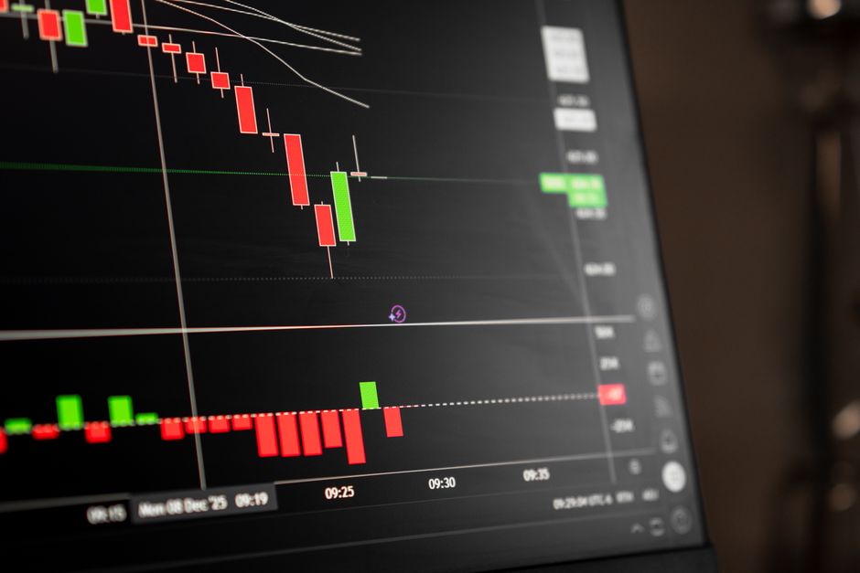
Calculation involves applying the Pearson correlation coefficient to the series of trade returns. A value near one indicates a trend in the equity curve, while a value near zero suggests independence. If the coefficient stays consistently positive, the strategy experiences streaks. This phenomenon is common when trading a specific fifteen minute range, as volatility clusters often persist through the morning. A sequence of trades taken during the regular trading hours should be analyzed for these shifts in dependency. If the autocorrelation shifts from positive to negative, the underlying market structure has changed.
Timeframe Sensitivity and Data Integrity
The choice of timeframe dictates the signal density. A 5 minute chart provides more data points for a statistical sample, but it also introduces more noise. Analyzing the equity curve produced by a 30 minute range requires a larger number of trades to reach statistical significance. Small sample sizes often produce false positives in autocorrelation tests. A sequence of ten trades is insufficient to prove a non-random edge. The data must span multiple sessions to ensure the pattern is not a byproduct of a single volatile market open.
Identifying Regime Shifts
Autocorrelation often breaks down when the market transitions between states. A strategy might show high positive correlation during a trending morning but shift to high negative correlation during the afternoon. Observing the equity curve during the transition from the premarket to the cash open helps isolate these shifts. If the correlation drops to zero, the mechanical advantage of the system is lost. Monitoring the session high and low against the trade sequence helps determine if the dependence is linked to specific price levels or time-based volatility.